Hurry Up Part 2

Filed in Cellular Automata | Game of Life Leave a comment

In Part 1 I showed that a lot of time is spent in the gol_defs updateState function indexing the neighbors to see who’s alive and who’s dead. For a 500 cell x 500 cell grid run for 50 cycles this accounts for 35% of the execution time. So much time is spent in this one location because the code is iterating over each cell in the grid, looking at the state of each neighbor and adding it to the count if it’s alive.

for neighbor in neighbors:
    # % does modulo indexing to create toroidal universe
    neighborR = (Rindex + neighbor[1]) % len(currentState)
    neighborC = (Cindex + neighbor[0]) % len(currentState[0])
    if currentState[neighborR][neighborC] == 1:
        count += 1

Since Python is an interpreted language this is a slow process but fortunately there are much faster ways to do the same thing. One way to speed this process up is to use an idea from image processing – convolution. This works by taking a small matrix, the kernel, and repeatedly applying it to each cell of a larger matrix in the following way. If the kernel is represented as:

a    b    c

d    e    f

g    h    i

and the larger grid is

A    B    C    D    E    F

G    H    I    J    K    L

M    N    O    P    Q    R

S    T    U    V    W    X

Then applying the kernel to cell H gives:

    Result = a*A + b*B + c*C + d*G + e*H + f*I + g*M + h*N + i*O

If the kernel is defined as

1    1    1

1    0    1

1    1    1

then for each cell we apply it to the result is the number of neighbors that are alive around the cell. The 0 in the middle keeps the cell itself from being counted. This is exactly what’s needed to calculate the number of neighbors so we can apply the game of life rules.

For instance if the grid contains

1    0    1    0

1    0    0    0

0    0    0    0

0    0    0    0

and we apply the kernel to the second cell in the second row from the top we get

Result = 1*1 + 0*1 + 1*1 + 1*1 + 0*0 + 0*1 + 0*1 + 0*1 + 0*1 = 3

which is the count of the number of alive neighbors. Since the count = 3 according to the game of life rules the cell will change from dead to alive.

The kernel is held in the neighbor variable in the main gol.py module. Now, instead of relative values used to calculate a neighbor index the variable will hold a 1 in each location that we want to consider as a neighbor. This kernel is then applied to each cell in the grid and used to calculate the number of alive neighbors.

So how is this faster? All I’ve done is replace a huge number of iterations with a huge number of iterations.
The difference is that I can now use SciPy which is a math, science and engineering library for Python that can speed up matrix operations tremendously. Replacing the existing code with a call to the Scipy convolve2d function does the convolution in a fraction of the time.

#Module import
import scipy.signal

# Function Definitions

def updateState(currentState, neighbors):
    nextState = copy.deepcopy(currentState)
    neighborCount = scipy.signal.convolve2d(currentState, neighbors, mode="same",boundary="wrap")
    Rindex = 0
    for row in neighborCount:
        Cindex = 0
        for cell in row:
            count = neighborCount[Rindex,Cindex]
            if count == 3:
                nextState[Rindex][Cindex] = 1
            elif count != (2 or 3):
                nextState[Rindex][Cindex] = 0
            Cindex += 1
        Rindex += 1
    return nextState

This takes the currentState grid, the neighbors kernel and convolves them to create a new matrix called neighborCount. Each cell in neighborCount contains the number of neighbors that are alive for that cell. Then all I have to do is iterate through neighborCount, read it and apply the game of life rules to find the next state of the cells in the grid. This happens much faster than the code in Hurry Up part 1. Now if I run the profiler I get the following (click to enlarge):
New Code:

output_new_cropped

Old Code:

  output_old_cropped

The new code only takes a little over 3% of the run time versus the 35% the old code took. So what does this mean for the overall run time? For 500 iterations I get:

                        New               Old            Improvement
100 cells x 100 cells =  10 seconds        15 seconds      33%
250 cells x 250 cells =  63 seconds        92 seconds      32% 
300 cells x 300 cells =  89 seconds       151 seconds      41%
500 cells x 500 cells = 243 seconds       393 seconds      38%

The improvement seen by the profiler shows up as a real improvement in the runtime. Notice that the improvement actually increases for larger grid sizes since the relative amount of time spent iterating over the grid is larger.

Getting better.

The next place to work on is in the update to the nextState array which again requires iterating through the whole array.

    Rindex = 0
    for row in neighborCount:
        Cindex = 0
        for cell in row:
            count = neighborCount[Rindex,Cindex]
            if count == 3:
                nextState[Rindex][Cindex] = 1
            elif count != (2 or 3):
                nextState[Rindex][Cindex] = 0
            Cindex += 1
        Rindex += 1

Using NumPy, which is part of SciPy, I can replace this with the NumPy where function.

    nextState[np.where(neighborCount == 3)] = 1
    nextState[np.where((neighborCount != 2) & (neighborCount != 3))] = 0
    return nextState                                               

The where function returns an array of indices of all cells that match the condition. These indices are then used to set the values of the cells in nextState. Of course to do this I had to go through and change all of the standard 2D lists I’ve been using into NumPy arrays but it was worth it. This and a few other small improvements result in (500 cycles):

                        New                Old            Improvement
100 cells x 100 cells =  1.2 seconds        15 seconds      92%
250 cells x 250 cells =  5.8  seconds       92 seconds      94% 
300 cells x 300 cells =  8.3  seconds      151 seconds      95%
500 cells x 500 cells = 22.4  seconds      393 seconds      94%

Amazon Web Services

Filed in EC2 | Game of Life | Linux 1 Comment

As mentioned previously Amazon offers services used by a lot of companies to provide affordable, scalable computing power. That’s great if you’re making money from whatever you’re doing on those servers. I’m not. So, what caught my eye is the AWS free usage tier. This gives you 750 hours of computing time each month for a year. Doing the math shows me that a month has about 750 hours so essentially you can have a server up and running continuously for free. Now this is what Amazon calls a micro instance so it’s not particularly fast or powerful but it’s still useful. I won’t repeat how to set up an account and an instance…you can read about that here. One thing I did differently is to just have a user name and password instead of of a key. No particular reason, just a preference. I can then SSH into the server from any computer or my mobile devices.

Once you’re up and running then you can do whatever you want with it. I uploaded my python modules using scp:

$ scp gol_ver2.0.py chad@54.203.101.174:~/projects/gol_ver2.0.py
$ scp gol_defs.py chad@54.203.101.174:~/projects/gol_defs.py

and then used SSH to log into the machine:

ssh -X chad@54.203.101.174

The -X turns on X forwarding so that I can use the graphical display option. For now though it’s glacially slow even for very small grids that result in small images. I’m not sure what’s going on there but I intend to find out. One thing I’ve tried is using compression and choosing a faster compression algorithm. It turns out that the default algorithm used by SSH is fairly slow. This is simple to change when you SSH in:

ssh -c arcfour,blowfish-cbc -XC chad@54.203.101.174

The arcfour and blowfish ciphers are quite a bit faster than the default though this didn’t really make a difference in the results I got. There’s some other problem slowing it down. I was kind of bummed about this (still am) but it got me to thinking about how to measure whether something interesting is happening in a game of life. That then goes back to the old question of what is life? It’s hard to define but you know it when you see it. Well, even if I could see it I don’t want to spend all my time staring at the monitor. The whole reason for doing this is so I can have a large universe running for long periods of time and just take a look at the interesting things when they occur. I’ll have to figure out how to measure things like the complexity of the grid, self organization and so on.

Hurry up, someone is waiting on you for that

Filed in Cellular Automata Leave a comment

The title of this post is from a fortune cookie I received a few years ago. I keep it on my desk at work to remind me not to waste time.

So what does this have to do with this blog? Well, now that I have a nice high resolution graphical display for my Game of Life program I’d like to be able to have runs with large numbers of cells. To some degree I can. Using the time command in a Linux terminal (time python yourprogram.py) with a Core i7 processor for 500 iterations I measured the following times for each run with no display and no sleep time between iterations:

100 cells x 100 cells =  15 seconds
250 cells x 250 cells =  92 seconds
300 cells x 300 cells = 151 seconds
500 cells x 500 cells = 393 seconds

Not bad but not exactly what I had in mind for an Autoverse. So how can I make it faster? The first thing to do is find out why it’s slow. For that we need to profile the code and see where it spends most of its time. Fortunately there are some tools to make it simple.

cProfile is a profiler that watches the code while it’s running and measures how long it spends in different areas.

$ python -m cProfile -o output.file gol.py

This results in a file that can be read using the pstats method

$ python
>>> import pstats
>>> p = pstats.Stats('output.file')

some things you can do with it then:

>>> p.strip_dirs().sort_stats(-1).print_stats()

strips out all the directory information and prints the results.
You can also sort by the total time and print out the top 10 time suckers:

>>> p.sort_stats('cumulative').print_stats(10)

What’s really nice though is to use Gprof2Dot to get a graph of the data.

$ python gprof2dot.py -f pstats output.file | dot -Tpng -o output.png

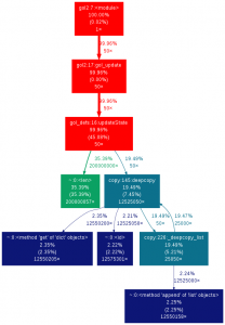
This is what it gave me (click to enlarge):
output

No great surprises here. The most time is spent in the gol_defs updateState function indexing the neighbors to see who’s alive and who’s dead. For a 500 cell x 500 cell grid run for 50 cycles this is done approximately 200 million times. 35% of the execution time is spent here. Seems like a good place to start.

Game of Life Graphical Display

Filed in Cellular Automata | Game of Life Leave a comment

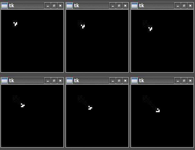
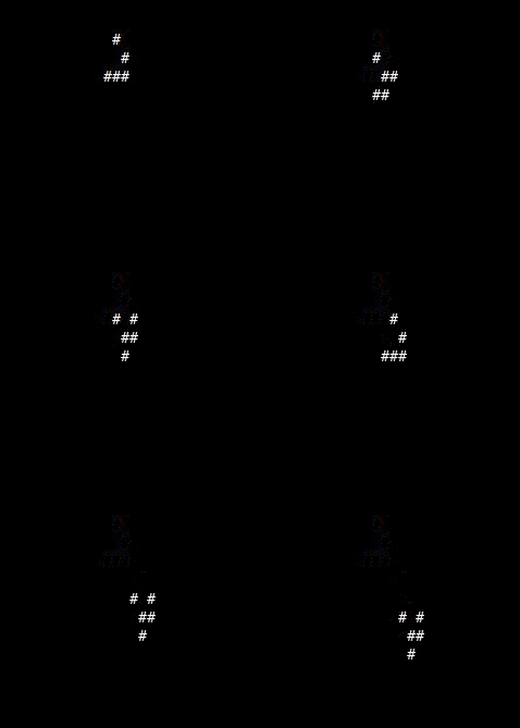
While the Game of Life ASCII display I talked about here is functional it’s limited and can’t show grids larger than a few dozen cells on a side. Fortunately Python has a standard module called Tkinter that allows for much better graphical displays. Using it requires a number of changes to the existing code but you get much nicer output. Compare the output of the graphical display with the old ASCII version.

graphical_glider                     my_glider


With the ASCII display I was able to implement it as a function that could be called as needed. Tkinter comes with it’s own event loop that handles updating the window and different events that might happen during operation. Tkinter windows have the ‘after’ method to schedule a function that is called after a certain number of milliseconds. The code that updates the state of the cells goes into this function.

For example:

#Module import
import Tkinter as tk

# Update function
def update(currentState):
    #this is where your code goes that does
    #whatever it is you want to do every
    #x milliseconds...100 for example
    currentState = newState
    #reset the after method to call update again in 100 ms
    root.after((100), update, currentState)

#Initialize
fps = 10 #number of times to update each second
# Create the root window 
root = tk.Tk()
#variable to hold image
tkimg = [None] 
tkimg[0] = state
#create label with image
label = tk.Label(root, image=tkimg[0])
label.pack(side="right")

#Run
root.after((1000/fps), gol_update, currentState)
root.mainloop() # main event handler


The images that are displayed are in PGM format. This format is very easy to use and allows for a simple transfer from array data to image data for display.

The functions to do so are defined in pgm_write.py. Currently I’m actually writing to a file which is then opened and displayed. This is not an efficient way to do this so I’ll change it soon to just store the image in a variable…but for now that’s the way it is.

# vim: tabstop=8 expandtab shiftwidth=4 softtabstop=4
'''
Chad Bonner Dec.19.2013
Game of Life PGM Image Write Function
pgm_write.py
'''
def write_file(image):
    #set up number of rows and colums variables from array size
    width = len(image[0])
    height = len(image)
    # define PGM Header
    pgmHeader = 'P5' + '\n' + str(width) + '  ' + str(height) + '  ' + str(1) + '\n'
    # open file for writing 
    filename = 'state.pgm'

    try:
        fout=open(filename, 'wb')
    except IOError, er:
        print "Cannot open file"
        sys.exit()

    # write the header to the file
    fout.write(pgmHeader)

    # write the data to the file 
    for row in image:
        for cell in row:
            #create byte for value of each cell
            pixel = chr(cell)  
            fout.write(pixel)
    # close the file
    fout.close()


To keep things from getting too unwieldy I took the functions used for the game of life mechanics and separated them into a different file gol_defs.py:

# vim: tabstop=8 expandtab shiftwidth=4 softtabstop=4
'''
Chad Bonner Dec.19.2013
Game of Life Function Definitions
gol_defs.py
'''
#Module import
import copy
import sys
import time
import random

# Function Definitions

def updateState(currentState, neighbors):
    '''
    this function is where the actual game of life calculations happen    
    for each cell
        count = 0
        for each neighbor
            if currentState == alive
                count = ++
        if count == 3
            nextState = alive
        else if count != 2 or 3
            nextState = dead
    '''
    nextState = copy.deepcopy(currentState)
    Rindex = 0
    for row in currentState:
        Cindex = 0
        for cell in row:
            count = 0
            for neighbor in neighbors:
                # % does modulo indexing to create toroidal universe
                neighborR = (Rindex + neighbor[1]) % len(currentState)
                neighborC = (Cindex + neighbor[0]) % len(currentState[0])
                if currentState[neighborR][neighborC] == 1:
                    count += 1
            if count == 3:
                nextState[Rindex][Cindex] = 1
            elif count != (2 or 3):
                nextState[Rindex][Cindex] = 0
            Cindex += 1
        Rindex += 1
    return nextState

def display(universe):
#very simple routine to display animated cell state in terminal
    sys.stderr.write("\x1b[2J\x1b[H")   #clear screen and reposition cursor
    for row in universe:
        for column in row:
            if column == 0:
                sys.stdout.write(' ') #leave empty for 0
            else: 
                sys.stdout.write('#') #fill in for 1 
        print "\r"
    sys.stdout.flush()

def populate(numR, numC, use_seed, insertR, insertC, seed):
    #populate either with a seed or with random 1s and 0s
    if use_seed == 0:
        #Populate with random field of 1s and 0s
        currentState = [[random.randint(0,1) for i in range(numC)] for j in range(numR)]
    else:
        #Populate with seed
        currentState = [[0 for i in range(numC)] for j in range(numR)]
        nextState = [[0 for i in range(numC)] for j in range(numR)]
        Cseed = len(seed[0])
        Rseed = len(seed)
        for i in range(Rseed):
            for j in range(Cseed):
                currentState[insertR+i][insertC+j] = seed[i][j]
    return currentState


This lets me concentrate on just the higher level display and control functions in the main module:

# vim: tabstop=8 expandtab shiftwidth=4 softtabstop=4
'''
Chad Bonner Dec.21.2013
Game of Life
gol.py
'''
#Module import
import Tkinter as tk
import sys
import time
import gol_defs
import pgm_write
import datetime

#GOL Update Loop
def gol_update(currentState):
    #update state with gol modulei
    currentState = gol_defs.updateState(currentState, neighbors) 
    #select display type
    if display == 3:
       #Display option 3 - graphical display
        pgm_write.write_file(currentState)
        #open state image
        state = tk.PhotoImage(file="state.pgm")
        #set image size
        width = dis_width/state.width()
        height = dis_height/state.height()
        state = state.zoom(width, height)
        tkimg[0] = state
        #update label with image
        label.configure(image = tkimg[0])
        root.after((1000/fps), gol_update, currentState)
    return currentState

#Declarations
run = True
rows = 250           #num rows of matrix
columns = 250        #num columns of matrix
fps = 10            #number of frames per second to display
sleepTime = 1.0/fps #calculate time to sleep between updates
use_seed = 0        #0=don't use seed, 1=use seed
display = 0         #0=no display, 1=info display, 2=ascii graphics, 3=tkinter
dis_width = 500      #display width and height 
dis_height = 500
#define locations of 8 neighbor cells
neighbors = [[-1,-1],[0,-1],[1,-1],[-1,0],[1,0],[-1,1],[0,1],[1,1]] 

seed = [[0,0,1],   #glider
        [1,0,1],
        [0,1,1]]

#Initialize
currentState = gol_defs.populate(rows, columns, use_seed, 3, 3, seed) 
root = tk.Tk()

#Initialize display according to display type selected
if display == 3:
    tkimg = [None] #used to keep image from being garbage collected
    pgm_write.write_file(currentState)
    state = tk.PhotoImage(file="state.pgm") #open state image
    #set image size
    width = dis_width/state.width()
    height = dis_height/state.height()
    state = state.zoom(width, height)
    tkimg[0] = state
    #create label with image
    label = tk.Label(root, image=tkimg[0])
    label.pack(side="right")
    #Run
    root.after((1000/fps), gol_update, currentState)
    root.mainloop()
else:
    while run == True:
        if display == 2:
            #display ASCII graphics
            gol_defs.display(currentState)
            currentState = gol_update(currentState)
            time.sleep(sleepTime)
        elif display == 1:
            #display info only
            print "working..."
            currentState = gol_update(currentState)
        else:
            #no display
            currentState = gol_update(currentState)

This is basically the same structure as in the cut down example above. What I’ve done here though is enable choosing the type of display to use. I want to choose between a graphical display, ASCII display, just printing useful information or no display at all for maximum speed. Since Tkinter requires initializing a window before it can do anything I decided to break the main loop into two parts. If I choose to use the graphical display then I use the after method of updating. If I choose one of the other display options then I use have to do my own looping with a while loop.

Game of Life

Filed in Cellular Automata | Game of Life 2 Comments

The Game of Life, created by John Conway in 1970, is probably the most well known cellular automata. Implemented on a grid it has a few very simple rules that are imposed at each cycle:

1. Any cell with fewer than two live neighbors dies
2. Any living cell with two or three living neighbors lives
3. Any living cell with more than three living neighbors dies
4. Any dead cell with exactly three living neighbors becomes a living cell
Continue Reading

Autoverse

Filed in Autoverse | Cellular Automata | EC2 Leave a comment

Recently I read Permutation City by Greg Egan and was intrigued by the concept of the Autoverse that plays a central role in the plot. The Autoverse is basically an artificial universe based on a cellular automaton and is complex enough to support a simplified chemistry used to create artificial life. The whole thing runs on distributed computing services that people rent time on.   The book was written in 1994 and in the meantime technology has kept marching on and provided us with an infrastructure very similar to what the Autoverse ran on in the form of the Internet and various computing providers such as Amazon’s EC2 service.

So, I’ll  be doing some projects here to learn more about cellular automata and using Amazon’s computers.

TOP